
强化学习随机游走
·
实现随机游走
1. gym环境:
random_walk.py
import io
import numpy as np
import sys
from gym.envs.toy_text import discrete

LEFT = 0
RIGHT = 1

class RandomWalkEnv(discrete.DiscreteEnv):
    """
    Random Walk environment

    T A B C(x) D E T
    x is your position and T are the two terminal states.
    """
    metadata = {'render.modes': ['human', 'ansi']}

    def __init__(self):

        shape = [1,7]

        self.shape = shape

        #  7个状态的状态空间
        nS = 7
        # 4个行为的行为空间
        nA = 2

        # 执行行为 a, 从状态s转移到状态s'的概率
        P = {}

        grid = np.arange(7).reshape(shape)
        it = np.nditer(grid, flags=['f_index'])

        while not it.finished:
            s = it.iterindex
            # 这里是一个字典的数组
            # 字典推导式
            P[s] = {a : [] for a in range(nA)}

            is_done = lambda s: s == 0 or s == (nS - 1)
            # 状态E,向左和向右的奖励不同
            reward = 0.0

            # 返回的 prob, next_state, reward, done
            # 得到当前状态执行一动作所得到的’反馈‘
            if is_done(s):
                P[s][LEFT] = [(1.0, s, reward, True)]
                P[s][RIGHT] = [(1.0, s, reward, True)]
            else:
                ns_left = int(s) - 1
                ns_right = int(s) + 1
                P[s][LEFT] = [(1.0, ns_left, reward, is_done(ns_left))]
                # 当当前状态为E时
                if s == nS - 2:
                    P[s][RIGHT] = [(1.0, ns_right, 1.0, is_done(ns_right))]
                else:
                    P[s][RIGHT] = [(1.0, ns_right, reward, is_done(ns_right))]

            it.iternext()

        # 选中状态空间中状态的概率
        isd = np.zeros(nS)
        # 状态 3 为开始状态
        isd[3] = 1.0
        self.P = P

        super(RandomWalkEnv, self).__init__(nS, nA, P, isd)

    def render(self, mode='human', close=False):
        self._render()

    def _render(self, mode='human', close=False):

        if close:
            return

        # io.StringIO(): 通过内存缓冲区实现文本的输入输出
        outfile = io.StringIO() if mode == 'ansi' else sys.stdout

        grid = np.arange(self.nS).reshape(self.shape)
        it = np.nditer(grid, flags=['multi_index'])

        while not it.finished:
            s = it.iterindex

            # 判断应该输出的字符
            if self.s == s:
                output = " {}(X) ".format(chr(ord('A') + self.s - 1))
            elif s == 0 or s == (self.nS - 1):
                output = " T "
            else:
                output = " {} ".format(chr(ord('A') + s - 1))

            outfile.write(output)
            if self.s == (self.nS - 1):
                outfile.write("\n")

            it.iternext()
2. 实现TD(0)算法和α\alphaαMC算法并进行比较
import warnings
from IPython.core.interactiveshell import InteractiveShell
warnings.filterwarnings("ignore")
InteractiveShell.ast_node_interactivity = "all"
import matplotlib.pyplot as plt
plt.rcParams['font.sans-serif'] = ['SimHei']  # 用来正常显示中文标签
plt.rcParams['axes.unicode_minus'] = False  # 用来正常显示负号
%matplotlib inline
import gym
import matplotlib
import numpy as np
import sys
import os

import itertools

from collections import defaultdict

par_dir = os.path.abspath(os.path.join(os.path.abspath('.'),os.path.pardir))
# 将父目录加入环境变量
if par_dir not in sys.path:
    sys.path.append(par_dir)

from lib.envs.random_walk import RandomWalkEnv

matplotlib.style.use('ggplot')
env = RandomWalkEnv()
α\alphaαMC算法
# 首次访问型蒙特卡洛算法
def mc_prediction(policy, env, num_episodes, alpha=0.5, discount_factor=1.0, batch=False):

#     returns_sum = defaultdict(float)
#     returns_count = defaultdict(float)
    V = {v: 0.5 if (v != 0 and v != env.nS - 1) else 0.0 for v in range(env.nS)}

    for i_episode in range(1, num_episodes + 1):

        # 每1000次输出一次进度
        if i_episode % 1000 == 0:
            print("\rEpisode {}/{}.".format(i_episode, num_episodes), end="")
            # 刷新输出缓冲区
            sys.stdout.flush()

        episode = []
        state = env.reset()
        for t in itertools.count():
            action = policy(state)
            next_state, reward, done, info = env.step(action)
            episode.append((state, action, reward))
            if done:
                break
            state = next_state

#         print(episode)
        states_in_episode = set([x[0] for x in episode])
        # 如果是批量更新
        if batch:
            for state in states_in_episode:
                # 返回迭代器的下一个项目
                first_occurence_idx = next(i for i,x in enumerate(episode) if x[0] == state)
                G = sum([x[2]*(discount_factor**i) for i,x in enumerate(episode[first_occurence_idx:])])
                V[state] = V[state] + alpha * (G - V[state])
        else:
            # 折扣收益总和
            G = 0.0
            for t in range(len(episode))[::-1]:
                state, action, reward = episode[t]
                G = discount_factor * G + reward
                V[state] = V[state] + alpha * (G - V[state])

    return V
# 选取行为的策略, 随机策略
def sample_policy(observation):

    # 状态 A~Z 向左和向右的概率为0.5
    action_probs = np.ones(env.nA) / env.nA
    action = np.random.choice(np.arange(env.nA), p=action_probs)
    return action if observation > 0 and  observation < (env.nS - 1) else None
V_mc = mc_prediction(sample_policy, env, num_episodes=1000)
Episode 1000/1000.
V_mc
{0: 0.0,
 1: 7.692724477211018e-06,
 2: 0.09277391436171792,
 3: 0.12109030039218549,
 4: 0.9987952634764677,
 5: 0.9839475434264258,
 6: 0.0}
TD(0)算法
# 一步时序差分预测算法
def td_zero(env, num_episodes, discount_factor=1.0, alpha=0.5, batch=False):

    V = {v: 0.5 if (v != 0 and v != env.nS - 1) else 0.0 for v in range(env.nS)}
    for i_episode in range(num_episodes):
        if (i_episode + 1) % 100 == 0:
            print("\rEpisode {}/{}.".format(i_episode + 1, num_episodes), end="")
            sys.stdout.flush()

        episode = []
        state = env.reset()
        for t in itertools.count():
            action = sample_policy(state)
            next_state, reward, done, info = env.step(action)
            episode.append((state, action, reward, next_state))
            if done:
                break
            state = next_state

        # 如果是批量更新
        states_in_episode = set([x[0] for x in episode])
        if batch:
            for state in states_in_episode:
                first_occurence_idx = next(i for i,x in enumerate(episode) if x[0] == state)
                state, action, reward, next_state = episode[first_occurence_idx]
                V[state] = V[state] + alpha*(reward + discount_factor*V[next_state] - V[state])
        else:
            for t in range(len(episode)):
                state, action, reward, next_state = episode[t]
                V[state] = V[state] + alpha*(reward + discount_factor*V[next_state] - V[state])

    return V
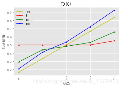
episode_nums = [1, 10, 100]
res = []
for num in episode_nums:
    V_td = td_zero(env, num_episodes=num, alpha=0.1)
    p = list(V_td.items())
    p.sort(key=lambda x: x[0])
    res.append(p)
Episode 100/100.
x = [chr(ord('A') + i) for i in range(5)]
real_y = [(i+1)/6 for i in range(5)]
plt.plot(x, real_y, 'y.-', label="real")

styles = ['r.-', 'g.-', 'b.-', 'c.-', 'm.-', 'y.-']

for i, val in enumerate(res):
    y = [val[1] for val in val][1:-1]
    plt.plot(x, y, styles[i], label=str(episode_nums[i]))

plt.xlabel("状态")
plt.ylabel("估计价值")
plt.title("TD(0)")

plt.legend()

plt.show()
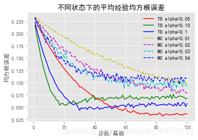
# 画出不同状态下的平均经验均方根误差
# TD步长参数[0.05, 0.15, 0.1], MC步长参数[0.01, 0.02, 0.03, 0.04]

line_styles = ['r', 'g', 'b', 'c', 'm', 'y']
dot_styles =  ['r--', 'g--', 'b--', 'c--', 'm--', 'y--'][::-1]

alphas = {
    'TD': [0.05, 0.15, 0.1],
    'MC': [0.01, 0.02, 0.03, 0.04]
}

mc_errors = []

# 每个状态的真实价值
x = np.arange(1, 101)
real_y = np.array([(i+1)/6 for i in range(5)])

for t in alphas.keys():
    print(t)
    # 分别求解求解 TD 算法和 MC 算法的均方根误差
    for s, alpha in enumerate(alphas[t]):

        # 所求误差是在100次运行中取5个状态上的平均误差的平均值
        current_errors = []
        for episode_num in range(100):

            print("\r{} 𝛼={} Episode num {}.".format(t, alpha, episode_num), end="")
            sys.stdout.flush()

            current_error = 0
            for i  in range(100):

                # 如果是时序差分算法
                if t == 'TD':
                    V = td_zero(env, num_episodes=episode_num + 1, alpha=alpha)
                else:
                    V = mc_prediction(sample_policy, env, num_episodes=episode_num + 1, alpha=alpha)

                current_y = np.array(list(map(lambda x:x[1], sorted(list(V.items())[1:-1], key=lambda x:x[0]))))

                # 求均方根误差
                err = np.sqrt(np.sum(np.power(real_y - current_y, 2)) / 5.0)
                # 增量更新平均值
                current_error += (1 / (i + 1)) * (err - current_error)

            current_errors.append(current_error)

        if t == 'TD':
            plt.plot(x, current_errors, line_styles[s], label="TD alpha={}".format(alpha))
        else:
            plt.plot(x, current_errors, dot_styles[s], label="MC alpha={}".format(alpha))


plt.xlabel("步数/幕数")
plt.ylabel("均方根误差")
plt.title("不同状态下的平均经验均方根误差")

plt.legend()

plt.show()
批量更新的随机游走
批量更新: 价值函数仅根据所有增量的和改变一次。然后利用新的值函数再次处理所有可用的经验,产生新的总增量,依此类推,直到价值函数收敛。
在批量更新下,只要选择足够小的步长参数α\alphaα, TD(0)就能确定地收敛到与α\alphaα无关的唯一结果。常数α\alphaαMC方法在相同条件下也能确定收敛,但是会收敛到不同的结果。
蒙特卡洛方法只是从某些有限的方面来说最优,而TD方法的最优性与预测回报这个任务更相关。
当α=0.01\alpha=0.01α=0.01,且训练幕数达到300时:
def batch_updating(t, iteration_num, alpha=0.01):
    current_errors = []
    real_y = np.array([(i+1)/6 for i in range(5)])
    for num_episode in range(100):

#         print("\r{} 𝛼={} Episode num {}.".format(t, alpha, num_episode), end="")
#         print("\r{} {} {}.".format(t, alpha, num_episode), end="")

        sys.stdout.flush()

        current_error = 0
        for i  in range(iteration_num):

            # 如果是时序差分算法
            if t == 'TD':
                V = td_zero(env, num_episodes=num_episode + 1, alpha=alpha, batch=True)
            else:
                V = mc_prediction(sample_policy, env, num_episodes=num_episode + 1, alpha=alpha, batch=True)

            current_y = np.array(list(map(lambda x:x[1], sorted(list(V.items())[1:-1], key=lambda x:x[0]))))

            # 求均方根误差
            err = np.sqrt(np.sum(np.power(real_y - current_y, 2)) / 5.0)
            # 增量更新平均值
            current_error += (1 / (i + 1)) * (err - current_error)

        current_errors.append(current_error)

    return current_errors
# 画出批量训练下, MC算法和TD算法在不同状态下的平均均方根误差

x = np.arange(1, 501)

td_errors = batch_updating('TD', 30)
mc_errors = batch_updating('MC', 30)

plt.plot(x, td_errors, label='TD')
plt.plot(x, mc_errors, label='MC')

plt.xlabel("步数/幕数")
plt.ylabel("不同状态下的平均均方根误差")

plt.legend()

plt.plot()
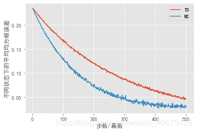
TD算法在批量更新时的表现在某些情况下能够好于MC算法,但不是所有的情况。
当TD算法的α=0.1\alpha=0.1α=0.1,MC算法的α=0.01\alpha=0.01α=0.01时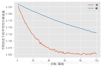
更多推荐


 0
0 0
0- 0


 已为社区贡献1条内容

所有评论(0)