刚入门深度学习，总听说“Attention is All You Need”却看不懂？别慌！这篇推文从核心概念到代码实现，手把手带你吃透Attention机制，零基础也能轻松入门～

另外我整理了相关论文+代码感兴趣的dd！

原文、姿.料 这里~

一、先搞懂：Attention机制到底是什么？

简单说，Attention机制模拟了人类的“注意力”——比如看一张照片时，你会重点关注人物，而非背景。
在深度学习中，它解决了传统模型（如RNN）“对所有输入一视同仁”的问题，能让模型自动给重要信息更高权重，不重要信息更低权重，从而提升任务效果（翻译、文本生成、图像识别都离不开它！）。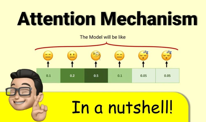

核心逻辑就3步：

1. 确定“哪些信息重要”（计算相似度）；
2. 给重要信息“打分”（归一化权重）；
3. 用权重整合信息（加权求和）。

二、核心公式：3步拆解Attention计算过程

以NLP中最基础的Scaled Dot-Product Attention（Transformer的核心）为例，先明确3个关键概念：

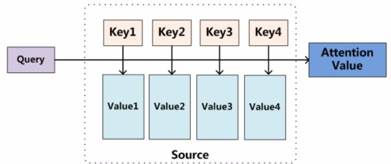
• Q (Query): 当前需要“关注”的对象（比如翻译时的当前单词）；
• K (Key): 所有待“被关注”的对象（比如原文中所有单词）；
• V (Value): 每个Key对应的具体信息（比如原文单词的语义向量）。
  

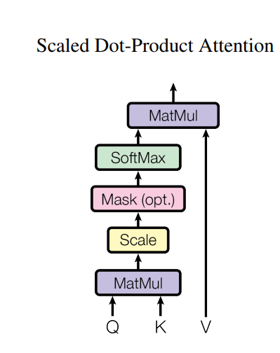
步骤1：计算Q与K的相似度（得分）

用“点积”衡量Q和K的关联程度，点积越大，说明两者越相关：
$$Score(Q,K)=Q\cdot K^T$$
（$K^T$是K的转置，确保矩阵维度可乘）

步骤2：缩放（避免梯度消失）

当K的维度（记为$d_k$）过大时，点积结果会飙升，导致Softmax后梯度消失。因此除以$\sqrt{d_k}$做缩放：
$$ScaledScore(Q,K)=\frac{Q\cdot K^T}{\sqrt{d_k}}$$

步骤3：掩码（可选，处理无效信息）

如果是文本生成等任务，需要屏蔽“未来时刻”的信息（比如翻译时不能提前看后面的单词），这一步会给无效位置加一个极小值（如$-1e9$）：
$$MaskedScore=Mask(ScaledScore(Q,K))$$

步骤4：归一化（得到权重）

用Softmax将得分转化为0-1之间的权重，确保所有权重和为1，权重越大表示该K越重要：
$$AttentionWeight=Softmax(MaskedScore)$$

步骤5：加权求和（得到最终注意力输出）

用权重对V进行加权，整合所有重要信息：
$$Attention(Q,K,V)=AttentionWeight\cdot V$$

三、代码实现：可直接运行的PyTorch版本

PyTorch已内置Attention相关工具，我们用最简单的代码实现“Scaled Dot-Product Attention”，新手复制就能跑！

1. 环境准备

先安装PyTorch（若已安装可跳过）：

pip install torch torchvision

2. 完整代码（含注释）

import torch
import torch.nn as nn
import torch.nn.functional as F
import matplotlib.pyplot as plt
import numpy as np
import os  # For creating directories and handling file paths

# ------------------- 1. Implement Scaled Dot-Product Attention -------------------
class ScaledDotProductAttention(nn.Module):
    def __init__(self):
        super().__init__()
        
    def forward(self, Q, K, V, mask=None):
        """
        Input parameters:
        - Q: [batch_size, num_heads, seq_len_q, d_k]  # Query vector
        - K: [batch_size, num_heads, seq_len_k, d_k]  # Key vector
        - V: [batch_size, num_heads, seq_len_v, d_v]  # Value vector (seq_len_k=seq_len_v by default)
        - mask: [batch_size, 1, seq_len_q, seq_len_k]  # Optional mask
        
        Output:
        - output: Attention-weighted result
        - attn_weight: Attention weights (for visualization)
        """
        d_k = Q.size(-1)
        # Step 1-2: Calculate scaled dot-product scores
        scores = torch.matmul(Q, K.transpose(-2, -1)) / torch.sqrt(torch.tensor(d_k, dtype=torch.float32))
        # Step 3: Apply mask if provided
        if mask is not None:
            scores = scores.masked_fill(mask == 0, -1e9)
        # Step 4: Get attention weights via Softmax
        attn_weight = F.softmax(scores, dim=-1)
        # Step 5: Weighted sum with Value
        output = torch.matmul(attn_weight, V)
        return output, attn_weight


# ------------------- 2. Visualization Functions (Save to File) -------------------
def plot_attention_heatmap(attn_weight, save_path, sample_idx=0, head_idx=0, seq_len=3):
    """
    Plot attention weight heatmap and SAVE to file (no popup)
    Args:
        save_path: Full path to save the heatmap (e.g., "./attention_heatmap.png")
    """
    # Extract weights of the specified sample and attention head
    weights = attn_weight[sample_idx, head_idx].detach().numpy()
    
    # Create heatmap
    plt.figure(figsize=(8, 6))
    ax = plt.gca()
    im = ax.imshow(weights, cmap='YlOrRd', aspect='auto')  # Darker = higher attention weight
    
    # Set labels and title
    ax.set_xlabel('Key Sequence Position', fontsize=12)
    ax.set_ylabel('Query Sequence Position', fontsize=12)
    ax.set_title(f'Attention Weight Heatmap (Sample {sample_idx+1}, Head {head_idx+1})', fontsize=14, pad=15)
    
    # Set tick marks (match sequence length)
    ax.set_xticks(np.arange(seq_len))
    ax.set_yticks(np.arange(seq_len))
    ax.set_xticklabels([f'K_{i+1}' for i in range(seq_len)])
    ax.set_yticklabels([f'Q_{i+1}' for i in range(seq_len)])
    
    # Add value annotations on each cell
    for i in range(seq_len):
        for j in range(seq_len):
            text = ax.text(j, i, f'{weights[i, j]:.2f}', ha='center', va='center', color='black', fontsize=10)
    
    # Add colorbar (explain weight intensity)
    cbar = plt.colorbar(im, ax=ax)
    cbar.set_label('Attention Weight (0=No Focus, 1=Full Focus)', fontsize=10)
    
    # Save to file (ensure high resolution)
    plt.tight_layout()
    plt.savefig(save_path, dpi=300, bbox_inches='tight')  # dpi=300 for high-quality image
    plt.close()  # Close figure to free memory (critical for server)
    print(f"✅ Attention heatmap saved to: {save_path}")


def plot_dimension_comparison(Q, K, V, output, save_path):
    """
    Plot dimension comparison bar chart and SAVE to file (no popup)
    Args:
        save_path: Full path to save the bar chart (e.g., "./dimension_comparison.png")
    """
    # Extract shape information
    q_shape = Q.shape
    k_shape = K.shape
    v_shape = V.shape
    out_shape = output.shape
    
    # Data for bar chart (focus on sequence length and feature dimension)
    metrics = ['Q Seq Len', 'K Seq Len', 'V Seq Len', 'Output Seq Len', 
               'Q Dim', 'K Dim', 'V Dim', 'Output Dim']
    values = [q_shape[2], k_shape[2], v_shape[2], out_shape[2], 
              q_shape[3], k_shape[3], v_shape[3], out_shape[3]]
    
    # Create bar chart
    plt.figure(figsize=(10, 6))
    bars = plt.bar(metrics, values, color=['skyblue', 'skyblue', 'skyblue', 'orange', 
                                           'lightgreen', 'lightgreen', 'lightgreen', 'orange'])
    
    # Add value labels on bars
    for bar, val in zip(bars, values):
        plt.text(bar.get_x() + bar.get_width()/2, bar.get_height() + 0.05, 
                 str(val), ha='center', va='bottom', fontsize=10)
    
    # Set labels and title
    plt.ylabel('Dimension Size', fontsize=12)
    plt.title('Dimension Comparison of Q/K/V and Attention Output', fontsize=14, pad=15)
    plt.ylim(0, max(values) + 1)  # Add margin for value labels
    plt.xticks(rotation=45)  # Rotate x-labels for readability
    
    # Save to file
    plt.tight_layout()
    plt.savefig(save_path, dpi=300, bbox_inches='tight')
    plt.close()  # Free memory
    print(f"✅ Dimension comparison chart saved to: {save_path}")


# ------------------- 3. Test & Auto-Save Results -------------------
if __name__ == "__main__":
    # --------------------------
    # Configuration (Modify here if needed)
    # --------------------------
    save_dir = "./attention_results"  # Directory to save images (auto-created if not exists)
    batch_size = 2
    num_heads = 2
    seq_len = 3
    d_k = d_v = 4
    
    # Step 1: Create save directory (avoid "file not found" errors)
    if not os.path.exists(save_dir):
        os.makedirs(save_dir)
        print(f"📂 Created save directory: {save_dir}")
    
    # Step 2: Simulate input data
    Q = torch.randn(batch_size, num_heads, seq_len, d_k)
    K = torch.randn(batch_size, num_heads, seq_len, d_k)
    V = torch.randn(batch_size, num_heads, seq_len, d_v)
    
    # Step 3: Simulate mask (block 3rd Key position, index=2)
    mask = torch.ones(batch_size, 1, seq_len, seq_len)
    mask[:, :, :, 2] = 0  # K_3 is invalid (weight → 0 after Softmax)
    
    # Step 4: Run Attention mechanism
    attention = ScaledDotProductAttention()
    output, attn_weight = attention(Q, K, V, mask)
    
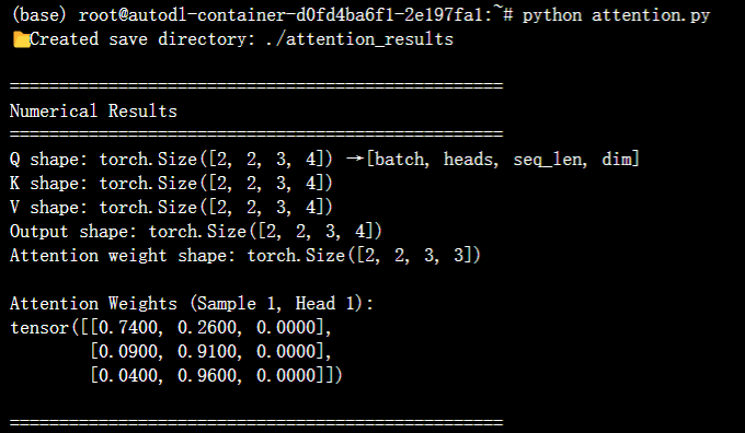
    # Step 5: Print numerical results (for debugging)
    print("\n" + "="*50)
    print("Numerical Results")
    print("="*50)
    print(f"Q shape: {Q.shape} → [batch, heads, seq_len, dim]")
    print(f"K shape: {K.shape}")
    print(f"V shape: {V.shape}")
    print(f"Output shape: {output.shape}")
    print(f"Attention weight shape: {attn_weight.shape}")
    print("\nAttention Weights (Sample 1, Head 1):")
    print(torch.round(attn_weight[0, 0] * 100) / 100)  # Round to 2 decimal places
    
    # Step 6: Define save paths for images
    heatmap_save_path = os.path.join(save_dir, "attention_heatmap.png")
    dim_chart_save_path = os.path.join(save_dir, "dimension_comparison.png")
    
    # Step 7: Generate and save plots (no popup)
    print("\n" + "="*50)
    print("Saving Visualization Results...")
    print("="*50)
    plot_attention_heatmap(attn_weight, heatmap_save_path, sample_idx=0, head_idx=0, seq_len=seq_len)
    plot_dimension_comparison(Q, K, V, output, dim_chart_save_path)
    
    # Final prompt
    print(f"\n🎉 All results saved successfully! Check images in: {os.path.abspath(save_dir)}")

3. 代码说明

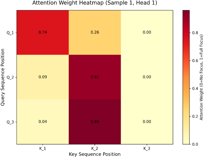
• 运行后会输出“注意力输出”和“注意力权重”，维度符合预期就说明成功；
• 权重矩阵中，值越大的位置，说明模型越关注该位置的信息；
• 掩码的作用是让模型“看不到”无效信息，比如文本中的padding（填充）部分。
  
  

四、新手必记：2个关键拓展

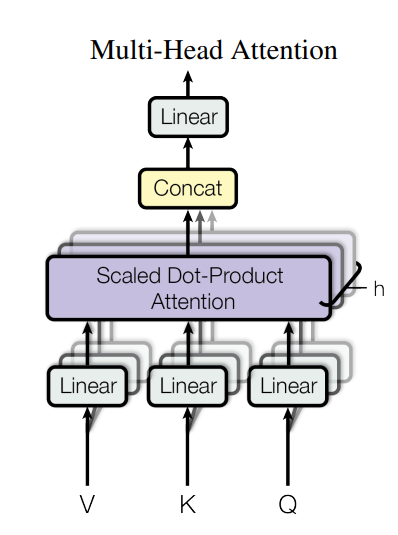
1. Multi-Head Attention（多头注意力）：
   刚才的代码中num_heads=2就是“多头”——把Q/K/V拆成多个头，每个头学习不同的注意力模式（比如一个头关注语法，一个头关注语义），最后再合并结果，效果比单头更好（Transformer的核心改进）。

2. Attention的应用场景：

   • NLP：机器翻译（如Google翻译）、文本摘要、聊天机器人；
   • CV：图像 caption（看图写文字）、目标检测（关注重点物体）；
   • 多模态：图文匹配（比如小红书图文检索）。

总结

Attention机制的核心就是“找重点、加权整合”，记住3个关键词（Q/K/V）和5步计算流程，再跑通代码，你就已经入门啦！
如果想深入，下一步可以学习Transformer结构（毕竟“Attention is All You Need”就是Transformer的论文标题），后续会继续更新～