学习率退火是一种策略，用于在训练过程中逐渐降低学习率，目的是提高模型的训练效果和收敛速度。这种方法通过在初始阶段采用较大学习率加速训练，而在接近优化的过程中降低学习率，以便进行更精细的调整和避免震荡。

1. 为什么要使用学习率退火？

        加速收敛：在训练的早期阶段，使用较大的学习率可以导致快速收敛，帮助模型迅速接近最优区域。
        避免震荡：随着训练进行，较小的学习率可以减少更新的振荡，使参数在最优解附近更加稳定。
        提高最终性能：通过在最后阶段使用较小的学习率，模型可以更好地精细调整参数，通常能得到更好的性能。

2. 学习率退火的策略

学习率退火有多种实现方式，以下是几种常见的策略：

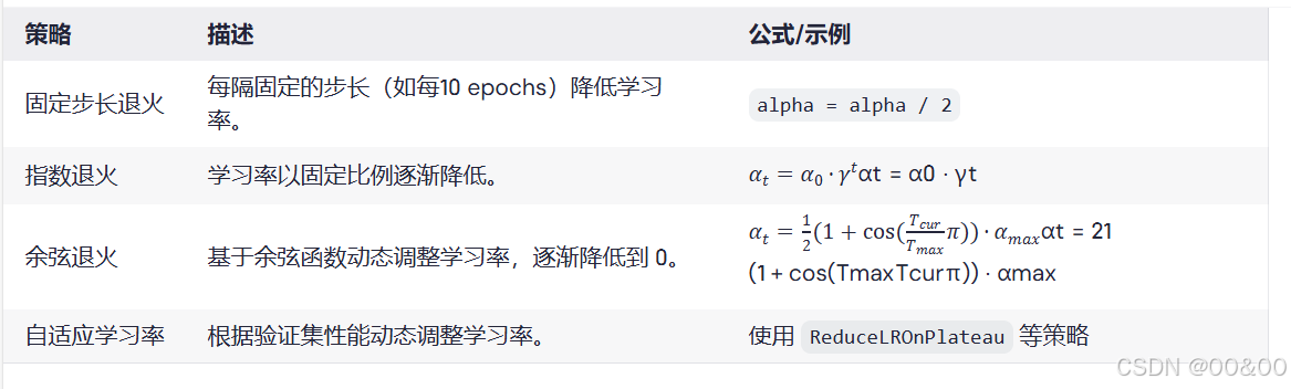
2.1 固定步长退火

        每个固定的迭代周期（如每10个epochs）降低学习率。例如，将学习率减半。

2.2 指数退火

        使用一个指数衰减公式：

        其中，是初始学习率，是衰减因子（通常小于1），是当前的epoch。

2.3 余弦退火

        使用余弦函数制定学习率：

        这里，是当前的epoch， 是总的epoch数。

2.4 自适应学习率

        使用动态调整学习率的方法，如ReduceLROnPlateau，根据验证集的性能动态调节学习率，当模型不再提升时降低学习率。

3. 实现学习率退火

在许多深度学习框架中（如Keras、PyTorch等），学习率退火的实现相对简单。以下是Keras中使用学习率调度器的示例：使用几种常见策略的比较及其代码实现。

3.1 不同的学习率退火策略

3.2 代码实现

下面是一个使用 Keras 的完整示例，比较几种学习率退火策略。

import numpy as np  
import matplotlib.pyplot as plt  
from tensorflow.keras.models import Sequential  
from tensorflow.keras.layers import Dense  
from tensorflow.keras.callbacks import ReduceLROnPlateau, LearningRateScheduler  
import tensorflow as tf  

# 生成模拟数据  
np.random.seed(0)  
X_train = np.random.rand(100, 2)  
y_train = (X_train[:, 0] ** 2 + X_train[:, 1] ** 2 > 1).astype(float)  # 二分类问题  

# 创建简单的模型  
def create_model():  
    model = Sequential()  
    model.add(Dense(64, activation='relu', input_dim=2))  
    model.add(Dense(1, activation='sigmoid'))  
    model.compile(optimizer='adam', loss='binary_crossentropy', metrics=['accuracy'])  
    return model  

# 1. 固定步长退火  
def fixed_step_decay(epoch, lr):  
    if epoch % 10 == 0 and epoch > 0:  
        lr *= 0.5  
    return lr  

# 设置固定步长退火  
model_fixed = create_model()  
callback_fixed = LearningRateScheduler(lambda epoch, lr: fixed_step_decay(epoch, lr))  

# 2. 指数退火  
def exponential_decay(epoch):  
    initial_lr = 0.01  
    k = 0.1  
    return initial_lr * np.exp(-k * epoch)  

# 设置指数退火  
model_exponential = create_model()  
callback_exponential = LearningRateScheduler(exponential_decay)  

# 3. 余弦退火  
def cosine_annealing(epoch):  
    T_max = 100  
    return 0.5 * (1 + np.cos(np.pi * epoch / T_max))  

# 设置余弦退火  
model_cosine = create_model()  
callback_cosine = LearningRateScheduler(cosine_annealing)  

# 4. 自适应学习率（ReduceLROnPlateau）  
model_adaptive = create_model()  
reduce_lr = ReduceLROnPlateau(monitor='val_loss', factor=0.5, patience=5, min_lr=1e-6)  

# 训练模型并记录学习率变化  
history_fixed = model_fixed.fit(X_train, y_train, epochs=100, callbacks=[callback_fixed], verbose=0)  
history_exponential = model_exponential.fit(X_train, y_train, epochs=100, callbacks=[callback_exponential], verbose=0)  
history_cosine = model_cosine.fit(X_train, y_train, epochs=100, callbacks=[callback_cosine], verbose=0)  
history_adaptive = model_adaptive.fit(X_train, y_train, epochs=100, validation_split=0.2, callbacks=[reduce_lr], verbose=0)  

# 绘制学习率变化  
plt.figure(figsize=(12, 6))  
plt.plot(history_fixed.history['lr'], label='Fixed Step Decay')  
plt.plot(history_exponential.history['lr'], label='Exponential Decay')  
plt.plot(history_cosine.history['lr'], label='Cosine Annealing')  
plt.plot(history_adaptive.history['lr'], label='Adaptive Learning Rate')  
plt.title('Learning Rate Strategy Comparison')  
plt.xlabel('Epoch')  
plt.ylabel('Learning Rate')  
plt.legend()  
plt.grid(True)  
plt.show()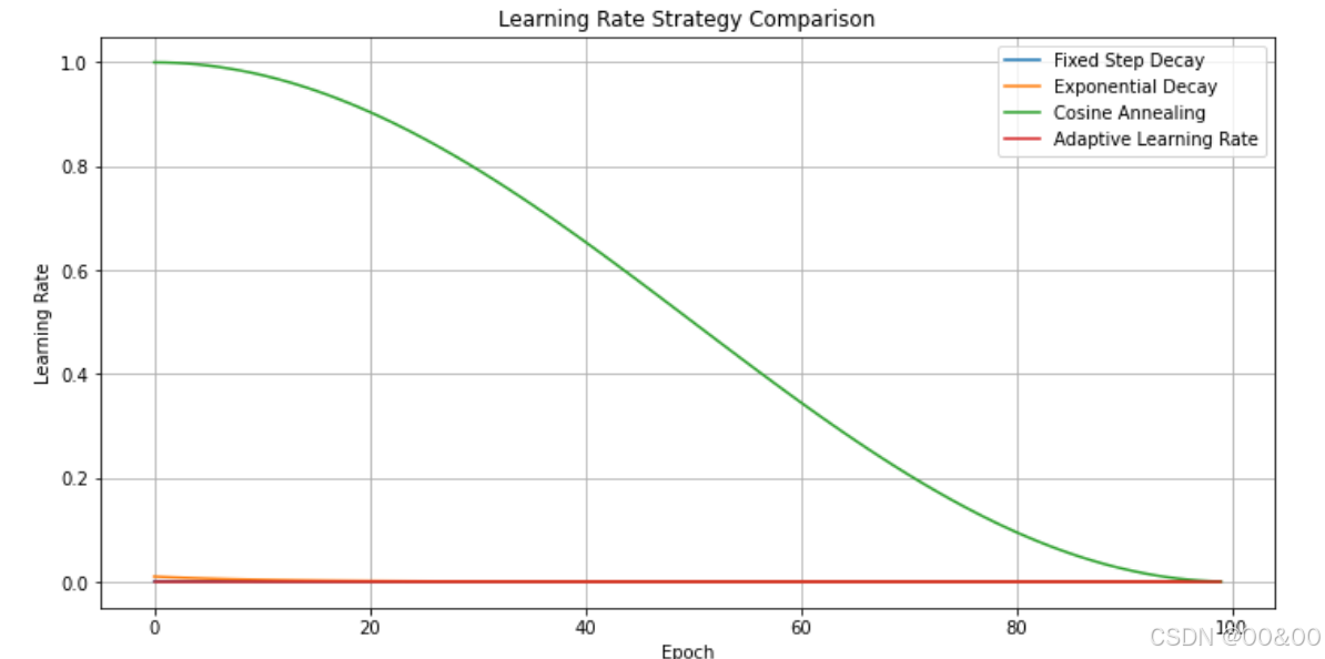

4. 总结

        学习率退火是优化深度学习模型的重要策略，可以有效提高模型的收敛性和最终性能。不同的退火策略适用于不同的任务和数据集。在选择学习率退火时，可以根据模型的训练情况进行微调。