
从零开始搭建深度学习大厦系列-1.深度学习基础(1-4)
说明:
(1)本人挑战手写代码验证理论,获得一些AI工具无法提供的收获和思考,对于一些我无法回答的疑问请大家在评论区指教;同时本系列文章有很多细节需要弄清楚,但是考虑到读者的吸收情况和文章篇幅限制,选择重点进行分享,如果有没说清楚或者解释错误的地方欢迎在评论区提出;
(2)如果需要进行复现或者调整,可以下载完整代码:移步个人空间的资源板块,对应的Py文件都有备注;
(3)由于许多内容来自本人课程报告,要求用英文撰写,这里就不翻译成中文了;
(4)本系列内容基于李沐老师《动手学深度学习》教材,网址:
《动手学深度学习》 — 动手学深度学习 2.0.0 documentation
同时提出了不同的代码实现方案和分析思路。本篇文章主要分析全连接层(FC)、多层感知机(MLP)超参数(HP)的作用原理和调整方法,以及数据预处理的方法。
Results of Textbook VS Mine
All of the four experiments are carried out on virtual environment based on Python interpreter 3.7.0 and mainly used packages include deep-learning package mxnet1.7.0.post2(CPU version), visualization package matplotlib.pyplot, data io package pandas.
Content
Optimization Methods(For Gradient Descent)
I、Simple Linear Regression Model
II、Single Layer Linear Regression(Fully Connected/Feed-Forword)
Learning Rate(numerator) Chosen For Adam_Full
Optimization Methods Comparison
III、Multiple Layers Perceptron & Fashion-MNIST
Results(Accuracy, Highest one)
IV、Kaggle House Price Prediction
Optimization Methods(For Gradient Descent)
def sgd(params,lr,batch_size):
    for param in params:
        print(param.grad)
        param[:]=param-lr*param.grad/batch_size
    return None,None

def sgd_momentum(params,lr,batch_size,momentums,lamb,r):
    for ind in range(len(params)):
        param=params[ind]
        momentum=momentums[ind]
        grad = param.grad + 2*r * batch_size * param
        momentum[:]=momentum*lamb+(1-lamb)*grad
        param[:]=param-lr*momentum/batch_size
    return momentums,None
def rms_prop(params,lr,batch_size,square_moments,rho,r,ch=1):
    for ind in range(len(params)):
        param=params[ind]
        s_m=square_moments[ind]
        grad = param.grad + 2*r * batch_size*param
        s_m[:]=s_m*rho+(1-rho)*(grad**2)
        if ch==1:
            param[:]=param-lr*param.grad/batch_size/(nd.sqrt(s_m)+1e-7)
        else:
            param[:]=param-lr*param.grad/batch_size/(nd.sqrt(s_m+1e-7))
    return None,square_moments
def adam_almost(params,lr,batch_size,momentums,square_moments,rho1,rho2,r):
for ind in range(len(params)):
param=params[ind]
m=momentums[ind]
grad=param.grad+2*r*batch_size*param
m[:]=m*rho1+(1-rho1)*grad
s_m=square_moments[ind]
s_m[:]=s_m*rho2+(1-rho2)*(grad**2)
param[:]=param-lr*m/batch_size/(nd.sqrt(s_m)+1e-7)
return momentums,square_moments
def adam_complete(params,lr,batch_size,momentums,square_moments,rho1,rho2,beta1,beta2,t,r):
for ind in range(len(params)):
param=params[ind]
m=momentums[ind]
grad=param.grad+2*r*batch_size*param
m[:]=m*rho1+(1-rho1)*grad
s_m=square_moments[ind]
s_m[:]=s_m*rho2+(1-rho2)*(grad**2)
unbias1=m/(1-beta1**t)
unbias2=s_m/(1-beta2**t)
param[:]=param-lr*unbias1/batch_size/(nd.sqrt(unbias2)+1e-7)
return momentums,square_moments# 网上关于丢弃法解读不一,李沐老师的实现是保证数学期望一致的丢弃法
# 李沐老师的实现思路在模型预测(test)的时候不需要继续丢弃
# 另一种实现是直接丢弃,保留参数不作/keep_prob处理,和adam_w 注释(2)本质类似
# 这种思路在预测时使用adam_w 注释 (2)的办法,确保训练和预测的一致性
def dropout(X, drop_prob):
assert 0 <= drop_prob <= 1
keep_prob = 1- drop_prob
# 这种情况下把全部元素都丢弃
if keep_prob == 0:
return X.zeros_like()
# mask = nd.random.uniform(0, 1, X.shape) > drop_prob
mask = nd.random.uniform(0, 1, X.shape) < keep_prob
return mask * X / keep_prob
# notice:this version of adam_w is not the authentic one!!!
# 由于网上没有搜集到合适的adam_w的解读资料,所以自己猜想了一下内部实现,
# 对于weight_decay的理解(1)每批数据权重更新添加drop out丢弃机制;
#(2)每批数据权重更新所有参数乘于小于1大于0的系数
def adam_w(params,lr,batch_size,momentums,square_moments,rho1,rho2,beta1,beta2,t,r,drop_r):
for ind in range(len(params)):
param=params[ind]
m=momentums[ind]
grad=param.grad+2*r*batch_size*param
m[:]=m*rho1+(1-rho1)*grad
s_m=square_moments[ind]
s_m[:]=s_m*rho2+(1-rho2)*(grad**2)
unbias1=m/(1-beta1**t)
unbias2=s_m/(1-beta2**t)
param[:]=param-lr*unbias1/batch_size/(nd.sqrt(unbias2)+1e-7)
# param[:]=(param-lr*unbias1/batch_size/(nd.sqrt(unbias2)+1e-7))*drop_r
# 此处和李沐老师的教材做法不同,没有在net函数内操作因此不需要判断是否正在训练模型,相当于在代码更里层丢弃
param[:]=dropout(param,drop_r)
return momentums,square_moments
I、Simple Linear Regression Model
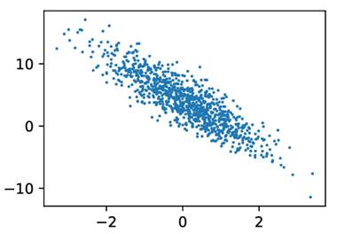
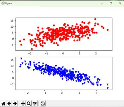
Figure 1 features(2 inputs) and labels, left comes from textbook
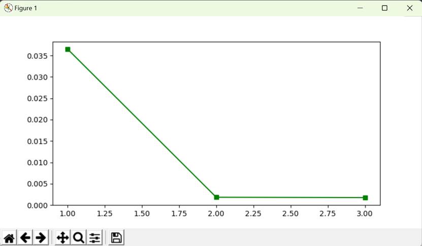
Figure 2 L2-loss and epochs——training curve
![]()
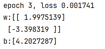
Figure 3 true/predicted weights(2x1) and bias(1)
Performance contrary: Hand designed version runs more slower than mxnet.gluon design(nn,gluon.Trainer).
II、Single Layer Linear Regression(Fully Connected/Feed-Forword)
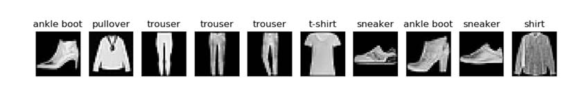
Figure 4 ten images demonstration (from dataset Fashion-MNIST,10 classes)
Results(Highest,Accuracy)
Training: 86.2%
Testing: 85.9%
Training Function(Shared with Part III)
# 模型训练
def train_epoches(tr_data_iter,net,loss,epoches,batch_size,params=None,lr=None,
fir_m=None,sec_m=None,rho1=None,rho2=None,beta1=None,beta2=None,decay_rate=None,lamb=None,r=None,trainer=None,te_data_iter=None):
losses = []
accs=[]
for epoch in range(epoches):
count=0
correct=0
train_l_sum=0
for X,y in tr_data_iter:
# 输入是float32,expected uint8(???)
# X=X.astype('uint8')
# 手动编程实现方法
# X=nd.cast(X,dtype=np.uint8)
X=X.astype('float32')
X=X.reshape(-1,784)
with autograd.record():
# Y_hat=softmax(net(X))
O_hat=net(X)
l=loss(O_hat,y).sum()
l.backward()
count+=len(y)
# print(f"len(y):{len(y)}")
if trainer is None:
lrt=lr/2*(1+np.cos(epoch/epoches*np.pi))
# sgd(params,lrt,len(y))
fir_m,_=sgd_momentum(params,lrt,len(y),fir_m,lamb,r)
# fir_m,sec_m=adam_w(params,lr,len(y),fir_m,sec_m,rho1,rho2,beta1,beta2,epoch+1,r,decay_rate)
# fir_m,sec_m=adam_complete(params,lr,len(y),fir_m,sec_m,rho1,rho2,beta1,beta2,epoch+1,r)
else:
trainer.step(batch_size)
# print(X.shape)
y = y.astype('float32')
correct+=int(accuracy(net,X,y)*len(y))
train_l_sum+=l.asscalar()
losses.append(train_l_sum/count)
test_acc=test_accuracy(te_data_iter,net)
print('epoch %d, loss %.4f, train acc %.3f, test acc %.3f'
% (epoch + 1, train_l_sum / count, correct / count, test_acc))
accs.append([correct/count,test_acc])
"""
if trainer is None:
print(f"epoch:{epoch + 1}:\n", params, "\n")
else:
print(f"epoch:{epoch + 1}:\n", net.collect_params(), "\n")
"""
accs=np.asarray(accs)
plt.figure()
plt.subplot(211)
plt.plot(range(epoches),losses,'b-o')
plt.title(f"sgd-momentum:{epoches, batch_size, lr, lamb, r}")
plt.subplot(212)
plt.plot(range(epoches),accs[:,0],'b-^',range(epoches),accs[:,1],'r-v')
plt.title(f"sgd-momentum:{epoches,batch_size,lr,lamb,r}")
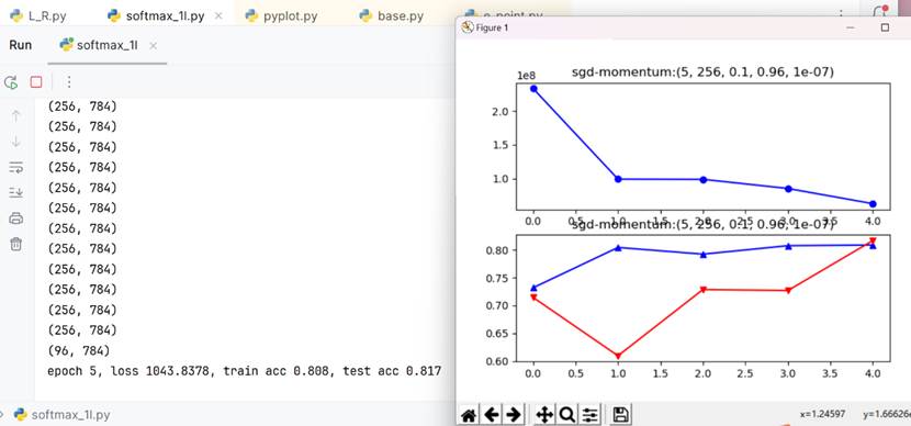
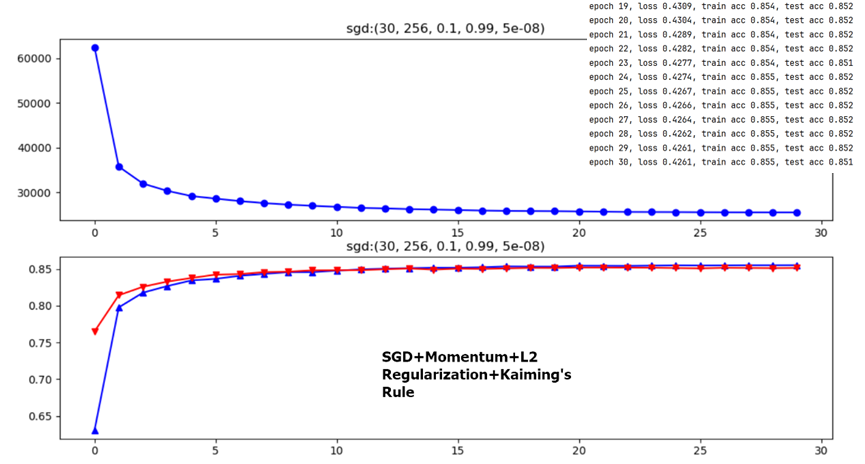
plt.show()Smaller Rho(in SGD+momentum)
Rho=0.9 or Rho=0.99 are two often chosen parameter values in momentum optimization. However, when Rho=0.9 it seems that overfitting occurs more often under same weight decay. So weight decay should be set larger for smaller Rho(0.9).
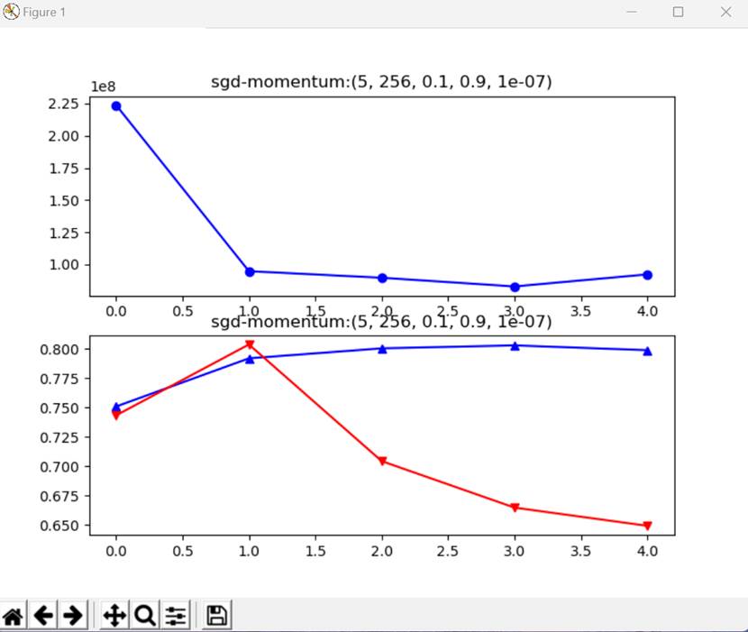
Figure 5 Overfitting(sgd+momentum), epochs-batch_size-learning rate-rho-weight decay
Data Preprocessing
It is extremely necessary to normalize the uint8 images into float32 ones(0-1), which belongs to data preprocessing mission.The following learing curves show the contrast with and without compressing the data range(domain). The loss of uint8-verison(unpreprocessed) isn’t divded by total sample amount and because of larger range distribution the divided loss is still far more larger than preprocessed verison. The unpreprocessed session may cause gradient explosion even if using gluon.SoftmaxCrossEntropy() to ensure value stability!
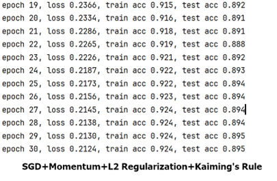
Notice: SGD+Momentum method includes L2 regularization controlled by parameter weight_decay(r) and learning rate decays among cosine curve.
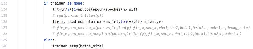
Figure 6 SGD+Momentum/Adam_full/SGD(/RMS_Prop/Adam_almost/”Adam_W”) coded by hand
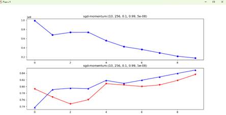
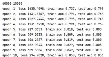
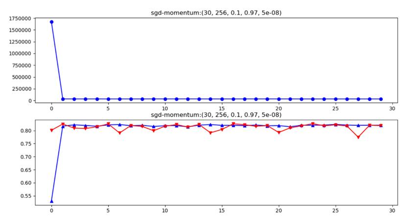
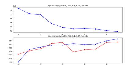
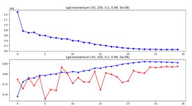
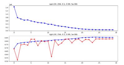
Figure 7 Swinging rapidly at the beginning due to uint8 inputs
Learning Rate(numerator) Chosen For Adam_Full
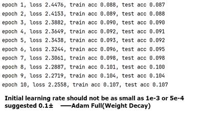
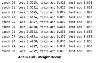
Figure 8 30 Epochs:Adam_Full+Weight Decay, learning rate(as numerator)=0.001(l) VS =0.1(r)
Optimization Methods Comparison
Adam full accommodates not so well as sgd+momentum method in 1-layer LR model, with -1.3% accuracy on testing dataset.

Initial Learning Rate
From the above two figures, it is obvious that lr=0.1 or lr=0.2 have no big difference with final testing accuracy only 0.8% deviation(initializing method are ineffective factors for 1-layer FC model here, see latter content).
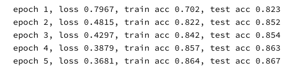
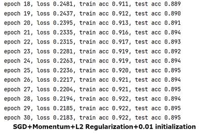
III、Multiple Layers Perceptron & Fashion-MNIST
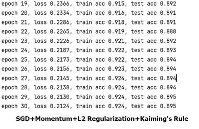
Results(Accuracy, Highest one)
Training: 92.4%
Testing: 89.5%
Model Structure
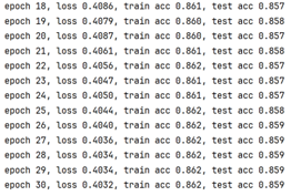
Two layer model(multiple layers perceptron, 1 hidden layer,784-256-10,relu as activation function) has +3.6% more accuracy than 1-layer FC but a bit worse generalization capacity than 1-layer FC model. See gap between training and testing dataset(6:1)——2.9% and 0.3% separately. However, this does not mean overfitting. Notice that initial learning rate(0.5) and weight decay(r) differ too.
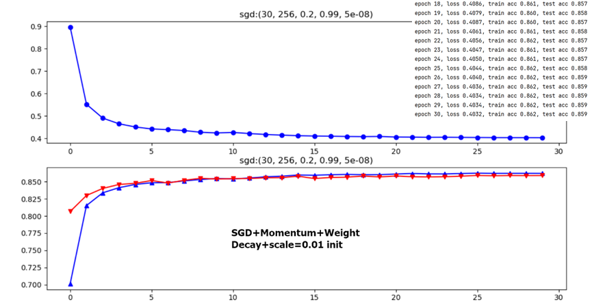
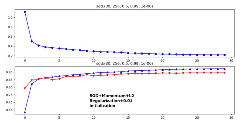
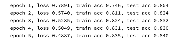
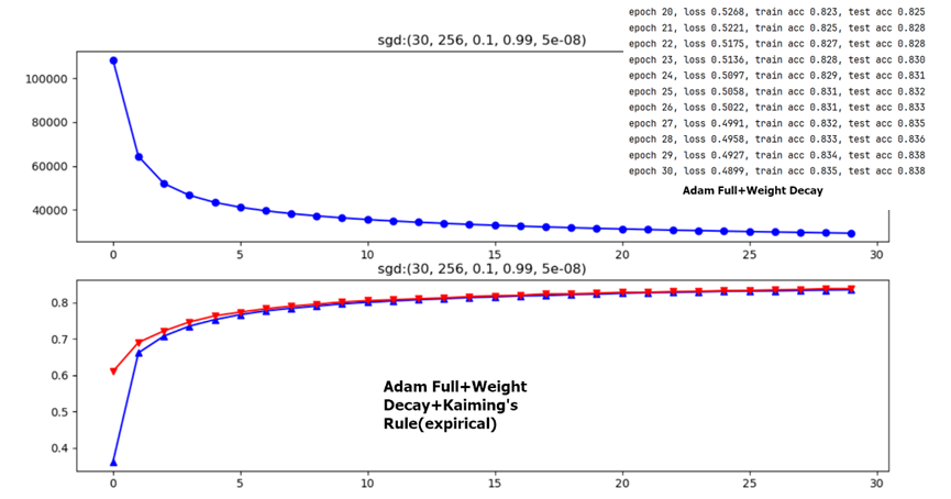
Figure 9 1-layer FC(784-10,up) VS multiple layers perceptron(784-256-10+RELU,down)
Weight Initialization
The following two figures dicuss different weight initialization methods in 1-layer FC network,it seems that for shallow NN Kaiming’s Rule doesn’t differ a lot from common expirical initialization method.
IV、Kaggle House Price Prediction
Data Preproessing
Besides those operations in textbook on features(331 at last)including one-hot encoding,standardization and nan values handling, it maybe also necessary to standardize the y label vector to train model and reverse the standardization operation after model prediction output to get true result (and to evaluate logarithm root mean square error properly), which is reasonable and this operaiton can be interpreted as one data preprocessing method.
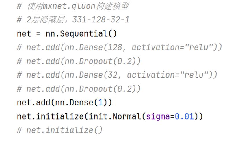
Figure 10 (Final) Model Structure For Part IV
Results(Loss)
5-fold cross validation(10 Epochs):0.1728253±0.0335098 0.20950612±0.01730189
5-fold cross validation(20 Epochs):0.11906052±0.00862629 0.16674939±0.01831708
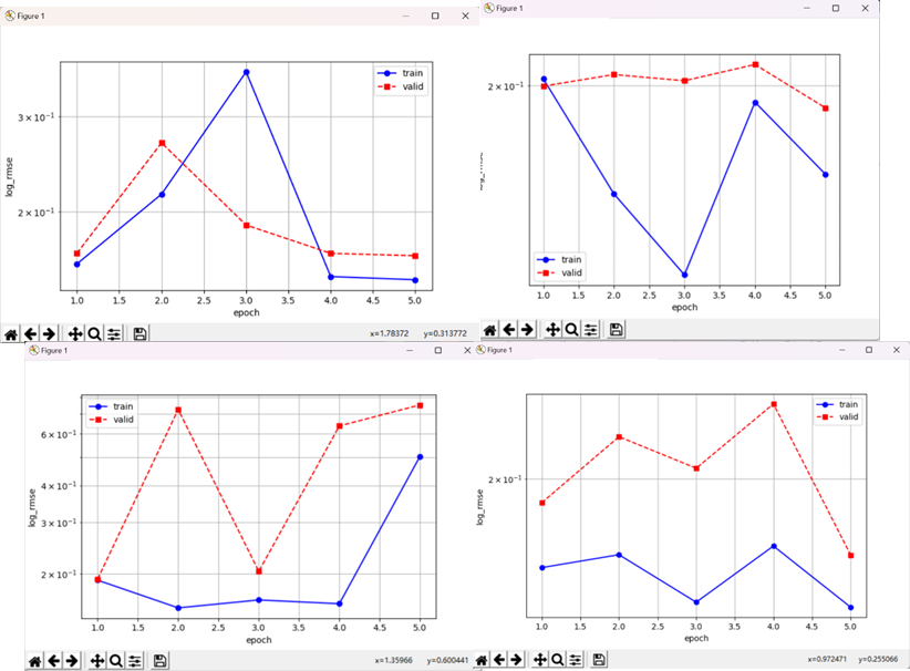
Figure 11 Visualize 5-fold cross validation(Epochs=10,lr=0.1,wd=0) loss(log_rmse) in 4 different trials
Epochs & Overfitting
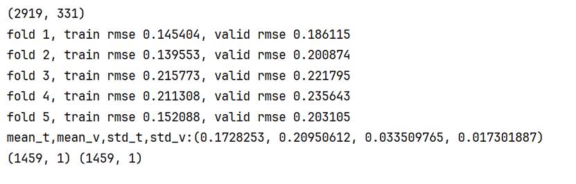
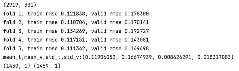
Figure 12 net: single layer FC optimize: Adam+lr=0.1+wd=0 epoches=10(up)/=20(down)
There may be overfitting caused by too many epochs of training, because when twenty epochs are set, much smaller variance of training loss in 5-fold cross-validation and bigger training-validation gap may be strong evidence indicating the guess.

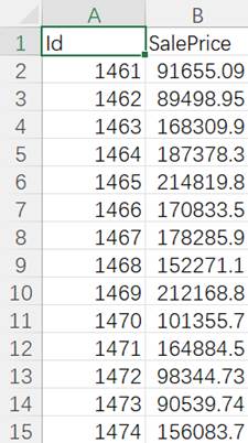
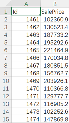
Figure 13 submission1/2/3.csv(prediction data output)
更多推荐


 10
10 0
0- 0


 已为社区贡献1条内容

所有评论(0)