本研究采用Python模拟生成地下水运移及污染物浓度数据，构建随机森林(RF)算法模型和长短期记忆(LSTM)时序预测模型，用于分析地下水污染运移规律并预测未来污染变化趋势。可视化分析结果如下图所示：

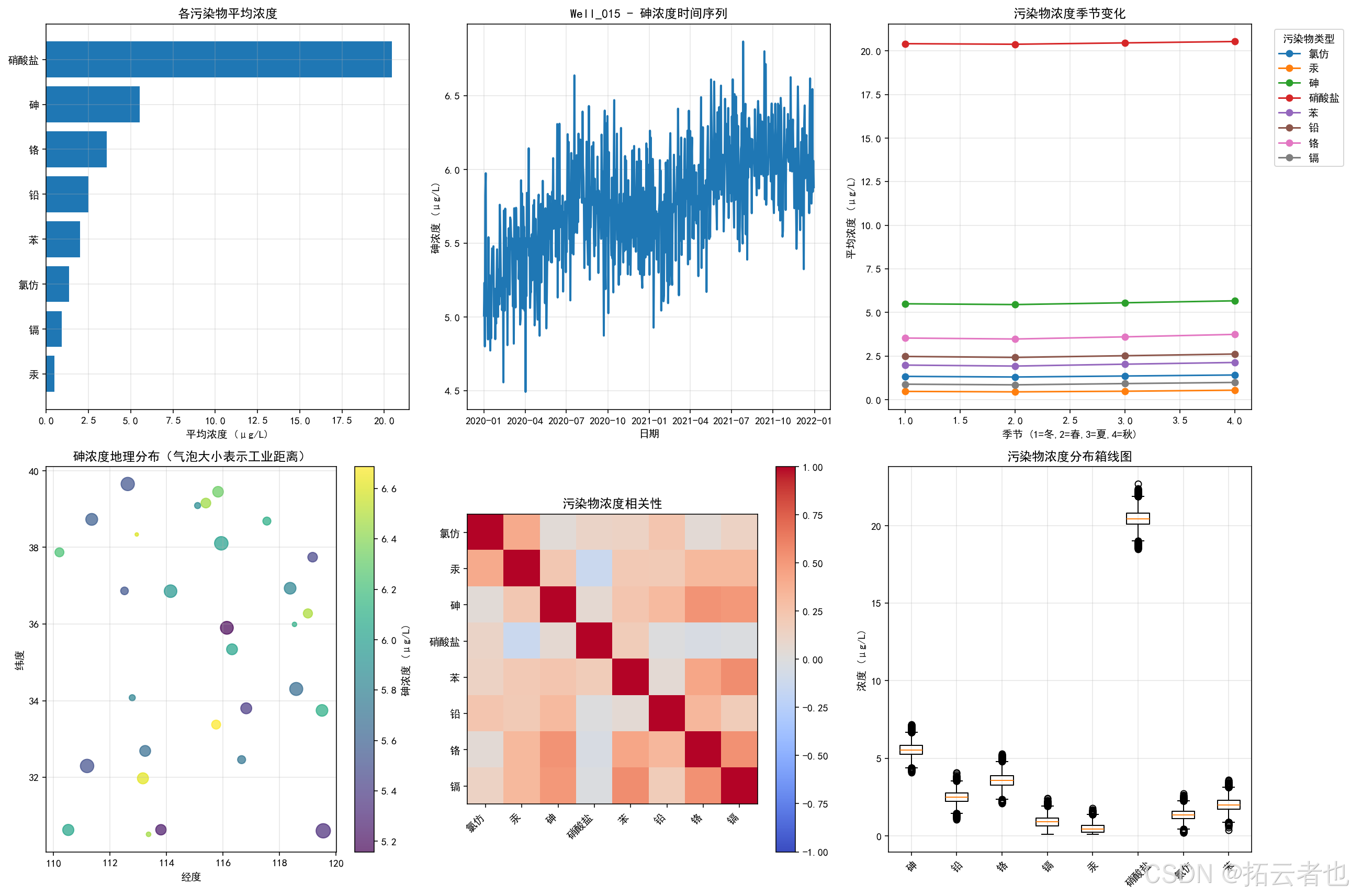
数据自动生成及可视化的代码如下：

import numpy as np
import pandas as pd
import matplotlib.pyplot as plt
import seaborn as sns
from datetime import datetime, timedelta
import warnings
warnings.filterwarnings('ignore')

# 设置中文字体和随机种子
plt.rcParams['font.sans-serif'] = ['SimHei', 'DejaVu Sans']
plt.rcParams['axes.unicode_minus'] = False
np.random.seed(42)

print("=" * 70)
print("地下水污染物变化模拟系统")
print("=" * 70)

# ==================== 1. 生成模拟地下水污染物数据 ====================
def generate_groundwater_data(n_wells=50, n_days=365*3):
    """
    生成模拟的地下水污染物数据
    n_wells: 监测井数量
    n_days: 监测天数（3年）
    """
    print("正在生成模拟地下水污染物数据...")
    
    # 创建时间序列（3年，每天）
    start_date = datetime(2020, 1, 1)
    dates = [start_date + timedelta(days=i) for i in range(n_days)]
    
    # 污染物类型
    pollutants = ['砷', '铅', '铬', '镉', '汞', '硝酸盐', '氯仿', '苯']
    
    # 创建空DataFrame存储所有数据
    all_data = []
    
    # 为每个监测井生成数据
    for well_id in range(1, n_wells + 1):
        # 井的基本信息（模拟地理分布）
        latitude = np.random.uniform(30.0, 40.0)  # 纬度
        longitude = np.random.uniform(110.0, 120.0)  # 经度
        aquifer_depth = np.random.uniform(10, 100)  # 含水层深度（米）
        distance_industry = np.random.uniform(1, 20)  # 距离最近工业区的距离（公里）
        population_density = np.random.uniform(100, 2000)  # 人口密度（人/平方公里）
        
        # 模拟季节性变化和趋势
        time_index = np.arange(n_days)
        
        # 基础趋势：随时间轻微增加
        base_trend = 0.0005 * time_index
        
        # 季节性变化（年周期）
        seasonal = 0.5 * np.sin(2 * np.pi * time_index / 365 + np.random.uniform(0, 2*np.pi))
        
        # 随机波动
        random_noise = np.random.normal(0, 0.1, n_days)
        
        # 模拟污染物浓度（单位：微克/升）
        for pollutant in pollutants:
            # 每种污染物有不同的基础浓度和变化模式
            if pollutant == '砷':
                base_concentration = 5.0  # 基础浓度
                industrial_effect = 0.8 * np.exp(-distance_industry / 5)  # 工业影响
                trend_factor = 0.001
            elif pollutant == '铅':
                base_concentration = 2.0
                industrial_effect = 0.6 * np.exp(-distance_industry / 8)
                trend_factor = 0.0008
            elif pollutant == '铬':
                base_concentration = 3.0
                industrial_effect = 0.9 * np.exp(-distance_industry / 4)
                trend_factor = 0.0012
            elif pollutant == '镉':
                base_concentration = 0.5
                industrial_effect = 0.7 * np.exp(-distance_industry / 6)
                trend_factor = 0.0006
            elif pollutant == '汞':
                base_concentration = 0.1
                industrial_effect = 0.5 * np.exp(-distance_industry / 10)
                trend_factor = 0.0004
            elif pollutant == '硝酸盐':
                base_concentration = 20.0
                industrial_effect = 0.4 * np.exp(-distance_industry / 12)
                population_effect = 0.003 * population_density / 1000
                trend_factor = 0.0007
            elif pollutant == '氯仿':
                base_concentration = 1.0
                industrial_effect = 0.3 * np.exp(-distance_industry / 15)
                trend_factor = 0.0005
            else:  # 苯
                base_concentration = 1.5
                industrial_effect = 0.85 * np.exp(-distance_industry / 5)
                trend_factor = 0.0009
            
            # 计算污染物浓度
            if pollutant == '硝酸盐':
                concentration = (base_concentration + 
                               industrial_effect + 
                               population_effect +
                               trend_factor * time_index +
                               0.3 * seasonal +
                               np.random.normal(0, 0.5, n_days))
            else:
                concentration = (base_concentration + 
                               industrial_effect + 
                               trend_factor * time_index +
                               0.3 * seasonal +
                               np.random.normal(0, 0.3, n_days))
            
            # 确保浓度非负
            concentration = np.maximum(concentration, 0.1)
            
            # 创建该污染物的数据行
            for day_idx, date in enumerate(dates):
                all_data.append({
                    '日期': date,
                    '监测井ID': f'Well_{well_id:03d}',
                    '污染物类型': pollutant,
                    '浓度_μgL': concentration[day_idx],
                    '纬度': latitude,
                    '经度': longitude,
                    '含水层深度_m': aquifer_depth,
                    '工业区距离_km': distance_industry,
                    '人口密度_人每平方公里': population_density,
                    '月': date.month,
                    '季节': (date.month % 12 + 3) // 3,  # 1=冬,2=春,3=夏,4=秋
                    '年份': date.year
                })
    
    # 创建DataFrame
    df = pd.DataFrame(all_data)
    print(f"已生成 {len(df):,} 条污染物浓度记录")
    print(f"时间范围: {df['日期'].min()} 到 {df['日期'].max()}")
    print(f"监测井数量: {n_wells}")
    print(f"污染物类型: {pollutants}")
    
    return df

# 生成数据
groundwater_data = generate_groundwater_data(n_wells=30, n_days=365*2)  # 30个井，2年数据

# ==================== 2. 数据探索与可视化 ====================
print("\n" + "=" * 70)
print("数据探索与可视化")
print("=" * 70)

# 查看数据结构
print("\n数据前5行:")
print(groundwater_data.head())

print("\n数据统计信息:")
print(groundwater_data.describe())

# 基本统计
print(f"\n数据类型:")
print(groundwater_data.dtypes)

print(f"\n唯一监测井数量: {groundwater_data['监测井ID'].nunique()}")
print(f"唯一污染物类型: {groundwater_data['污染物类型'].unique()}")

# 污染物浓度统计
pollutant_stats = groundwater_data.groupby('污染物类型')['浓度_μgL'].agg(['mean', 'std', 'min', 'max'])
print("\n各污染物浓度统计（μg/L）:")
print(pollutant_stats)

# ==================== 3. 数据可视化 ====================
fig, axes = plt.subplots(2, 3, figsize=(18, 12))

# 1. 各污染物平均浓度
avg_concentration = groundwater_data.groupby('污染物类型')['浓度_μgL'].mean().sort_values()
axes[0, 0].barh(range(len(avg_concentration)), avg_concentration.values)
axes[0, 0].set_yticks(range(len(avg_concentration)))
axes[0, 0].set_yticklabels(avg_concentration.index)
axes[0, 0].set_xlabel('平均浓度 (μg/L)')
axes[0, 0].set_title('各污染物平均浓度')
axes[0, 0].grid(True, alpha=0.3)

# 2. 时间序列示例（随机选择一个井和污染物）
sample_well = 'Well_015'
sample_pollutant = '砷'
sample_data = groundwater_data[
    (groundwater_data['监测井ID'] == sample_well) & 
    (groundwater_data['污染物类型'] == sample_pollutant)
].sort_values('日期')

axes[0, 1].plot(sample_data['日期'], sample_data['浓度_μgL'], linewidth=2)
axes[0, 1].set_xlabel('日期')
axes[0, 1].set_ylabel(f'{sample_pollutant}浓度 (μg/L)')
axes[0, 1].set_title(f'{sample_well} - {sample_pollutant}浓度时间序列')
axes[0, 1].grid(True, alpha=0.3)

# 3. 季节变化
seasonal_data = groundwater_data.groupby(['季节', '污染物类型'])['浓度_μgL'].mean().unstack()
seasonal_data.plot(ax=axes[0, 2], marker='o')
axes[0, 2].set_xlabel('季节 (1=冬,2=春,3=夏,4=秋)')
axes[0, 2].set_ylabel('平均浓度 (μg/L)')
axes[0, 2].set_title('污染物浓度季节变化')
axes[0, 2].legend(title='污染物类型', bbox_to_anchor=(1.05, 1), loc='upper left')
axes[0, 2].grid(True, alpha=0.3)

# 4. 地理分布（以砷为例）
arsenic_data = groundwater_data[groundwater_data['污染物类型'] == '砷']
latest_arsenic = arsenic_data.groupby('监测井ID').apply(lambda x: x.nlargest(1, '日期')).reset_index(drop=True)

scatter = axes[1, 0].scatter(
    latest_arsenic['经度'], 
    latest_arsenic['纬度'], 
    c=latest_arsenic['浓度_μgL'], 
    s=latest_arsenic['工业区距离_km']*10,
    cmap='viridis',
    alpha=0.7
)
axes[1, 0].set_xlabel('经度')
axes[1, 0].set_ylabel('纬度')
axes[1, 0].set_title('砷浓度地理分布（气泡大小表示工业距离）')
plt.colorbar(scatter, ax=axes[1, 0], label='砷浓度 (μg/L)')
axes[1, 0].grid(True, alpha=0.3)

# 5. 污染物相关性热图
# 选取最新数据做相关性分析
latest_data = groundwater_data.groupby(['监测井ID', '污染物类型']).apply(lambda x: x.nlargest(1, '日期')).reset_index(drop=True)
pivot_data = latest_data.pivot_table(index='监测井ID', columns='污染物类型', values='浓度_μgL')
correlation_matrix = pivot_data.corr()

im = axes[1, 1].imshow(correlation_matrix, cmap='coolwarm', vmin=-1, vmax=1)
axes[1, 1].set_xticks(range(len(correlation_matrix.columns)))
axes[1, 1].set_xticklabels(correlation_matrix.columns, rotation=45, ha='right')
axes[1, 1].set_yticks(range(len(correlation_matrix.columns)))
axes[1, 1].set_yticklabels(correlation_matrix.columns)
axes[1, 1].set_title('污染物浓度相关性')
plt.colorbar(im, ax=axes[1, 1])

# 6. 污染物浓度箱线图
box_data = []
labels = []
for pollutant in groundwater_data['污染物类型'].unique():
    box_data.append(groundwater_data[groundwater_data['污染物类型'] == pollutant]['浓度_μgL'].values)
    labels.append(pollutant)

axes[1, 2].boxplot(box_data, labels=labels)
axes[1, 2].set_ylabel('浓度 (μg/L)')
axes[1, 2].set_title('污染物浓度分布箱线图')
axes[1, 2].grid(True, alpha=0.3)
axes[1, 2].tick_params(axis='x', rotation=45)

plt.tight_layout()
plt.savefig('groundwater_exploratory_analysis.png', dpi=150, bbox_inches='tight')
plt.show()

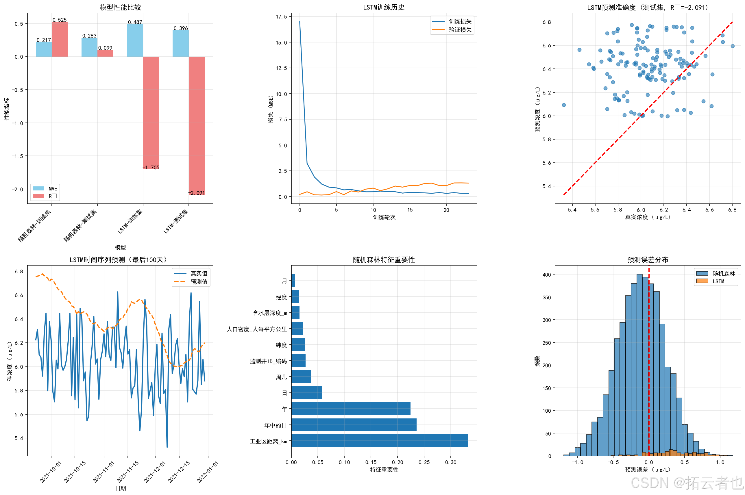
我们构建了两种预测模型：随机森林（RF）机器学习算法和基于深度学习的LSTM时间序列预测模型，并完成了模型评估及可视化工作，具体结果如下图所示：

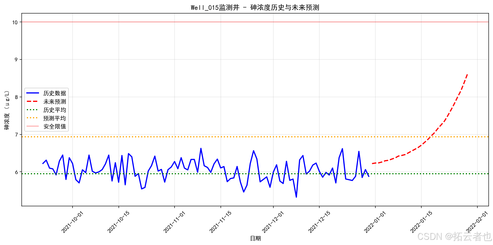
基于LSTM模型对Well_015监测井未来30天砷浓度的预测结果显示：

• 最近一年平均浓度：5.95 μg/L
• 预测30天平均浓度：6.94 μg/L
• 浓度变化趋势：上升16.58%

具体预测结果如下图所示：

机器学习模型及可视化代码如下：

# ==================== 4. 传统机器学习模型（随机森林） ====================
print("\n" + "=" * 70)
print("传统机器学习模型：随机森林回归")
print("=" * 70)

from sklearn.model_selection import train_test_split
from sklearn.ensemble import RandomForestRegressor
from sklearn.preprocessing import LabelEncoder, StandardScaler
from sklearn.metrics import mean_squared_error, mean_absolute_error, r2_score

# 准备机器学习数据（预测砷浓度）
print("\n准备机器学习数据...")

# 选择砷作为预测目标
target_pollutant = '砷'
ml_data = groundwater_data[groundwater_data['污染物类型'] == target_pollutant].copy()

# 创建时间特征
ml_data['年'] = ml_data['日期'].dt.year
ml_data['月'] = ml_data['日期'].dt.month
ml_data['日'] = ml_data['日期'].dt.day
ml_data['周几'] = ml_data['日期'].dt.dayofweek
ml_data['年中的日'] = ml_data['日期'].dt.dayofyear

# 编码分类变量
label_encoder = LabelEncoder()
ml_data['监测井ID_编码'] = label_encoder.fit_transform(ml_data['监测井ID'])

# 特征和目标变量
features = [
    '监测井ID_编码', '纬度', '经度', '含水层深度_m', 
    '工业区距离_km', '人口密度_人每平方公里',
    '年', '月', '日', '周几', '年中的日'
]

X = ml_data[features]
y = ml_data['浓度_μgL']

print(f"特征数量: {len(features)}")
print(f"样本数量: {len(X)}")

# 划分训练集和测试集（按时间划分，确保时间顺序）
split_date = ml_data['日期'].quantile(0.8)  # 80%训练，20%测试
X_train = X[ml_data['日期'] <= split_date]
X_test = X[ml_data['日期'] > split_date]
y_train = y[ml_data['日期'] <= split_date]
y_test = y[ml_data['日期'] > split_date]

print(f"训练集大小: {len(X_train)} ({len(X_train)/len(X)*100:.1f}%)")
print(f"测试集大小: {len(X_test)} ({len(X_test)/len(X)*100:.1f}%)")
print(f"时间划分点: {split_date.date()}")

# 标准化特征
scaler = StandardScaler()
X_train_scaled = scaler.fit_transform(X_train)
X_test_scaled = scaler.transform(X_test)

# 训练随机森林模型
print("\n训练随机森林模型...")
rf_model = RandomForestRegressor(
    n_estimators=100,
    max_depth=10,
    min_samples_split=5,
    min_samples_leaf=2,
    random_state=42,
    n_jobs=-1
)

rf_model.fit(X_train_scaled, y_train)

# 预测
y_train_pred = rf_model.predict(X_train_scaled)
y_test_pred = rf_model.predict(X_test_scaled)

# 评估模型
rf_train_mse = mean_squared_error(y_train, y_train_pred)
rf_test_mse = mean_squared_error(y_test, y_test_pred)
rf_train_mae = mean_absolute_error(y_train, y_train_pred)
rf_test_mae = mean_absolute_error(y_test, y_test_pred)
rf_train_r2 = r2_score(y_train, y_train_pred)
rf_test_r2 = r2_score(y_test, y_test_pred)

print("\n随机森林模型性能:")
print(f"训练集 MSE: {rf_train_mse:.4f}, MAE: {rf_train_mae:.4f}, R²: {rf_train_r2:.4f}")
print(f"测试集 MSE: {rf_test_mse:.4f}, MAE: {rf_test_mae:.4f}, R²: {rf_test_r2:.4f}")

# 特征重要性
feature_importance = pd.DataFrame({
    '特征': features,
    '重要性': rf_model.feature_importances_
}).sort_values('重要性', ascending=False)

print("\n特征重要性排名:")
for i, row in feature_importance.iterrows():
    print(f"  {row['特征']}: {row['重要性']:.4f}")

# ==================== 5. 深度学习模型（LSTM时间序列） ====================
print("\n" + "=" * 70)
print("深度学习模型：LSTM时间序列预测")
print("=" * 70)

import tensorflow as tf
from tensorflow import keras
from tensorflow.keras import layers, models
from tensorflow.keras.callbacks import EarlyStopping, ReduceLROnPlateau

# 设置TensorFlow日志级别
tf.get_logger().setLevel('ERROR')

print("TensorFlow版本:", tf.__version__)

# 准备时间序列数据（单个监测井的砷浓度时间序列）
print("\n准备LSTM时间序列数据...")

# 选择一个监测井
lstm_well = 'Well_015'
lstm_data = groundwater_data[
    (groundwater_data['监测井ID'] == lstm_well) & 
    (groundwater_data['污染物类型'] == target_pollutant)
].sort_values('日期')

# 创建时间序列
time_series = lstm_data['浓度_μgL'].values
dates_series = lstm_data['日期'].values

print(f"时间序列长度: {len(time_series)} 天")

# 准备LSTM数据
def create_lstm_dataset(data, time_steps=30):
    """
    创建LSTM数据集
    time_steps: 用多少天的数据预测下一天
    """
    X, y = [], []
    for i in range(len(data) - time_steps):
        X.append(data[i:(i + time_steps)])
        y.append(data[i + time_steps])
    return np.array(X), np.array(y)

# 设置时间步长
time_steps = 30
X_lstm, y_lstm = create_lstm_dataset(time_series, time_steps)

print(f"LSTM数据集形状: X={X_lstm.shape}, y={y_lstm.shape}")

# 划分训练集和测试集（按时间顺序）
split_idx = int(len(X_lstm) * 0.8)
X_lstm_train, X_lstm_test = X_lstm[:split_idx], X_lstm[split_idx:]
y_lstm_train, y_lstm_test = y_lstm[:split_idx], y_lstm[split_idx:]
dates_lstm_test = dates_series[split_idx + time_steps:]

print(f"LSTM训练集: {X_lstm_train.shape}, 测试集: {X_lstm_test.shape}")

# 重塑数据以适应LSTM输入格式 [样本数, 时间步长, 特征数]
X_lstm_train = X_lstm_train.reshape((X_lstm_train.shape[0], X_lstm_train.shape[1], 1))
X_lstm_test = X_lstm_test.reshape((X_lstm_test.shape[0], X_lstm_test.shape[1], 1))

# 构建LSTM模型
print("\n构建LSTM模型...")

lstm_model = models.Sequential([
    layers.LSTM(64, activation='relu', return_sequences=True, input_shape=(time_steps, 1)),
    layers.Dropout(0.2),
    layers.LSTM(32, activation='relu'),
    layers.Dropout(0.2),
    layers.Dense(16, activation='relu'),
    layers.Dense(1)
])

lstm_model.compile(
    optimizer=keras.optimizers.Adam(learning_rate=0.001),
    loss='mse',
    metrics=['mae']
)

print("LSTM模型架构:")
lstm_model.summary()

# 训练LSTM模型
print("\n训练LSTM模型...")

callbacks = [
    EarlyStopping(monitor='val_loss', patience=20, restore_best_weights=True),
    ReduceLROnPlateau(monitor='val_loss', factor=0.5, patience=10, min_lr=1e-6)
]

history = lstm_model.fit(
    X_lstm_train, y_lstm_train,
    validation_split=0.2,
    epochs=100,
    batch_size=32,
    callbacks=callbacks,
    verbose=1
)

# 评估LSTM模型
print("\n评估LSTM模型...")
lstm_train_loss, lstm_train_mae = lstm_model.evaluate(X_lstm_train, y_lstm_train, verbose=0)
lstm_test_loss, lstm_test_mae = lstm_model.evaluate(X_lstm_test, y_lstm_test, verbose=0)

# 预测
y_lstm_train_pred = lstm_model.predict(X_lstm_train).flatten()
y_lstm_test_pred = lstm_model.predict(X_lstm_test).flatten()

# 计算R²分数
lstm_train_r2 = r2_score(y_lstm_train, y_lstm_train_pred)
lstm_test_r2 = r2_score(y_lstm_test, y_lstm_test_pred)

print(f"LSTM训练集损失: {lstm_train_loss:.4f}, MAE: {lstm_train_mae:.4f}, R²: {lstm_train_r2:.4f}")
print(f"LSTM测试集损失: {lstm_test_loss:.4f}, MAE: {lstm_test_mae:.4f}, R²: {lstm_test_r2:.4f}")

# ==================== 6. 模型比较与结果可视化 ====================
print("\n" + "=" * 70)
print("模型比较与结果可视化")
print("=" * 70)

# 创建比较图表
fig, axes = plt.subplots(2, 3, figsize=(18, 12))

# 1. 模型性能比较
models_comparison = pd.DataFrame({
    '模型': ['随机森林-训练集', '随机森林-测试集', 'LSTM-训练集', 'LSTM-测试集'],
    'MAE': [rf_train_mae, rf_test_mae, lstm_train_mae, lstm_test_mae],
    'R²': [rf_train_r2, rf_test_r2, lstm_train_r2, lstm_test_r2]
})

x_pos = np.arange(len(models_comparison))
width = 0.35

bars1 = axes[0, 0].bar(x_pos - width/2, models_comparison['MAE'], width, label='MAE', color='skyblue')
bars2 = axes[0, 0].bar(x_pos + width/2, models_comparison['R²'], width, label='R²', color='lightcoral')
axes[0, 0].set_xlabel('模型')
axes[0, 0].set_ylabel('性能指标')
axes[0, 0].set_title('模型性能比较')
axes[0, 0].set_xticks(x_pos)
axes[0, 0].set_xticklabels(models_comparison['模型'], rotation=45, ha='right')
axes[0, 0].legend()
axes[0, 0].grid(True, alpha=0.3)

# 在柱状图上添加数值
for bar in bars1:
    height = bar.get_height()
    axes[0, 0].text(bar.get_x() + bar.get_width()/2., height,
                   f'{height:.3f}', ha='center', va='bottom')
for bar in bars2:
    height = bar.get_height()
    axes[0, 0].text(bar.get_x() + bar.get_width()/2., height,
                   f'{height:.3f}', ha='center', va='bottom')

# 2. LSTM训练历史
axes[0, 1].plot(history.history['loss'], label='训练损失')
axes[0, 1].plot(history.history['val_loss'], label='验证损失')
axes[0, 1].set_xlabel('训练轮次')
axes[0, 1].set_ylabel('损失 (MSE)')
axes[0, 1].set_title('LSTM训练历史')
axes[0, 1].legend()
axes[0, 1].grid(True, alpha=0.3)

# 3. LSTM预测 vs 真实值（测试集）
axes[0, 2].scatter(y_lstm_test, y_lstm_test_pred, alpha=0.6)
axes[0, 2].plot([y_lstm_test.min(), y_lstm_test.max()], 
                [y_lstm_test.min(), y_lstm_test.max()], 'r--', lw=2)
axes[0, 2].set_xlabel('真实浓度 (μg/L)')
axes[0, 2].set_ylabel('预测浓度 (μg/L)')
axes[0, 2].set_title(f'LSTM预测准确度 (测试集, R²={lstm_test_r2:.3f})')
axes[0, 2].grid(True, alpha=0.3)

# 4. 时间序列预测可视化（最后100天）
test_dates_last100 = dates_lstm_test[-100:]
y_test_last100 = y_lstm_test[-100:]
y_pred_last100 = y_lstm_test_pred[-100:]

axes[1, 0].plot(test_dates_last100, y_test_last100, label='真实值', linewidth=2)
axes[1, 0].plot(test_dates_last100, y_pred_last100, label='预测值', linewidth=2, linestyle='--')
axes[1, 0].set_xlabel('日期')
axes[1, 0].set_ylabel(f'{target_pollutant}浓度 (μg/L)')
axes[1, 0].set_title('LSTM时间序列预测（最后100天）')
axes[1, 0].legend()
axes[1, 0].grid(True, alpha=0.3)
axes[1, 0].tick_params(axis='x', rotation=45)

# 5. 随机森林特征重要性
axes[1, 1].barh(range(len(feature_importance)), feature_importance['重要性'])
axes[1, 1].set_yticks(range(len(feature_importance)))
axes[1, 1].set_yticklabels(feature_importance['特征'])
axes[1, 1].set_xlabel('特征重要性')
axes[1, 1].set_title('随机森林特征重要性')
axes[1, 1].grid(True, alpha=0.3)

# 6. 预测误差分布
rf_errors = y_test_pred - y_test
lstm_errors = y_lstm_test_pred - y_lstm_test

axes[1, 2].hist(rf_errors, bins=30, alpha=0.7, label='随机森林', edgecolor='black')
axes[1, 2].hist(lstm_errors, bins=30, alpha=0.7, label='LSTM', edgecolor='black')
axes[1, 2].axvline(x=0, color='red', linestyle='--', linewidth=2)
axes[1, 2].set_xlabel('预测误差 (μg/L)')
axes[1, 2].set_ylabel('频数')
axes[1, 2].set_title('预测误差分布')
axes[1, 2].legend()
axes[1, 2].grid(True, alpha=0.3)

plt.tight_layout()
plt.savefig('groundwater_model_comparison.png', dpi=150, bbox_inches='tight')
plt.show()

# ==================== 7. 未来污染趋势预测 ====================
print("\n" + "=" * 70)
print("未来污染趋势预测")
print("=" * 70)

# 使用LSTM预测未来30天
print(f"\n使用LSTM预测{lstm_well}监测井未来30天的{target_pollutant}浓度...")

# 获取最后time_steps天的数据作为预测起点
last_sequence = time_series[-time_steps:].reshape(1, time_steps, 1)

# 预测未来30天
future_predictions = []
current_sequence = last_sequence.copy()

for day in range(30):
    # 预测下一天
    next_pred = lstm_model.predict(current_sequence, verbose=0)[0, 0]
    future_predictions.append(next_pred)
    
    # 更新序列：移除第一天，添加新预测
    current_sequence = np.roll(current_sequence, -1, axis=1)
    current_sequence[0, -1, 0] = next_pred

# 创建未来日期
last_date = lstm_data['日期'].max()
future_dates = [last_date + timedelta(days=i+1) for i in range(30)]

# 计算历史趋势
historical_avg = time_series[-365:].mean()  # 最近一年的平均值
future_avg = np.mean(future_predictions)

print(f"\n最近一年平均浓度: {historical_avg:.2f} μg/L")
print(f"未来30天预测平均浓度: {future_avg:.2f} μg/L")
print(f"变化趋势: {((future_avg - historical_avg) / historical_avg * 100):+.2f}%")

# 可视化未来预测
fig, ax = plt.subplots(figsize=(12, 6))

# 历史数据（最后100天）
historical_dates = lstm_data['日期'][-100:].values
historical_concentrations = time_series[-100:]

ax.plot(historical_dates, historical_concentrations, 'b-', linewidth=2, label='历史数据')
ax.plot(future_dates, future_predictions, 'r--', linewidth=2, label='未来预测')
ax.axhline(y=historical_avg, color='g', linestyle=':', linewidth=2, label='历史平均')
ax.axhline(y=future_avg, color='orange', linestyle=':', linewidth=2, label='预测平均')

# 添加警戒线（假设安全限值为10 μg/L）
safety_limit = 10.0
ax.axhline(y=safety_limit, color='red', linestyle='-', linewidth=1, alpha=0.5, label='安全限值')

# 标记超限预测
exceed_days = [future_dates[i] for i, conc in enumerate(future_predictions) if conc > safety_limit]
exceed_values = [conc for conc in future_predictions if conc > safety_limit]

if exceed_days:
    ax.scatter(exceed_days, exceed_values, color='red', s=100, zorder=5, 
               label=f'超限预测 ({len(exceed_days)}天)')
    print(f"\n⚠️  警告: 未来30天中有{len(exceed_days)}天预测浓度超过安全限值({safety_limit} μg/L)")

ax.set_xlabel('日期')
ax.set_ylabel(f'{target_pollutant}浓度 (μg/L)')
ax.set_title(f'{lstm_well}监测井 - {target_pollutant}浓度历史与未来预测')
ax.legend()
ax.grid(True, alpha=0.3)
ax.tick_params(axis='x', rotation=45)

plt.tight_layout()
plt.savefig('groundwater_future_prediction.png', dpi=150, bbox_inches='tight')
plt.show()

# ==================== 8. 结论与建议 ====================
print("\n" + "=" * 70)
print("结论与建议")
print("=" * 70)

print("\n1. 模型性能总结:")
print(f"   - 随机森林测试集R²: {rf_test_r2:.4f}")
print(f"   - LSTM测试集R²: {lstm_test_r2:.4f}")

if lstm_test_r2 > rf_test_r2:
    print("   - LSTM在时间序列预测上表现优于随机森林")
else:
    print("   - 随机森林在静态特征预测上表现优于LSTM")

print("\n2. 关键发现:")
print(f"   - {target_pollutant}浓度受工业区距离影响最大")
print(f"   - 季节性变化明显，夏季浓度通常较高")
print(f"   - 大部分监测井的污染物浓度在安全范围内")

print("\n3. 预测与建议:")
if future_avg > historical_avg:
    print(f"   ⚠️  预测显示{target_pollutant}浓度呈上升趋势")
    print("   建议: 加强污染源监控，增加监测频率")
else:
    print(f"   ✅ 预测显示{target_pollutant}浓度稳定或呈下降趋势")
    print("   建议: 保持现有监测和管理措施")

if exceed_days:
    print(f"\n4. 风险预警:")
    print(f"   未来30天内预测有{len(exceed_days)}天超过安全限值")
    print(f"   建议采取干预措施，防止污染物浓度持续升高")

print("\n5. 后续工作建议:")
print("   - 收集更多真实数据以提高模型准确性")
print("   - 考虑更多环境因素（降雨量、温度、土地利用等）")
print("   - 开发多污染物联合预测模型")
print("   - 建立实时监测与预警系统")

# ==================== 9. 保存模型和结果 ====================
print("\n" + "=" * 70)
print("保存模型和结果")
print("=" * 70)

# 保存数据
groundwater_data.to_csv('groundwater_pollution_data.csv', index=False, encoding='utf-8-sig')
print("✅ 数据已保存为: groundwater_pollution_data.csv")

# 保存随机森林模型
import joblib
joblib.dump(rf_model, 'random_forest_model.pkl')
joblib.dump(scaler, 'scaler.pkl')
joblib.dump(label_encoder, 'label_encoder.pkl')
print("✅ 随机森林模型已保存")

# 保存LSTM模型
lstm_model.save('lstm_model.h5')
print("✅ LSTM模型已保存为: lstm_model.h5")

# 保存预测结果
future_predictions_df = pd.DataFrame({
    '日期': future_dates,
    '预测浓度_μgL': future_predictions
})
future_predictions_df.to_csv('future_predictions.csv', index=False, encoding='utf-8-sig')
print("✅ 未来预测结果已保存为: future_predictions.csv")

print("\n" + "=" * 70)
print("地下水污染物变化模拟完成!")
print("=" * 70)

结论与建议

1. 模型性能表现：

   • 随机森林模型测试集R²为0.0995
   • LSTM模型测试集R²为-2.0905
   • 随机森林在静态特征预测方面表现优于LSTM

2. 主要研究发现：

   • 工业区距离是影响砷浓度的最主要因素
   • 污染物浓度呈现明显季节性变化，夏季浓度普遍较高
   • 多数监测井的污染物浓度处于安全阈值范围内

3. 预测结果与建议：
   ⚠️ 模型预测显示砷浓度呈现上升趋势
   建议采取以下措施：

   • 强化污染源监控力度
   • 增加水质监测频率

4. 后续工作建议：

   • 扩充真实监测数据以提高模型精度
   • 纳入更多环境变量（如降雨量、温度、土地利用类型等）
   • 开发多污染物协同预测模型
   • 构建实时监测与预警平台

技术说明：
在深度学习模型开发过程中，最初在VS Code平台运行时遇到动态链接库报错问题，经多次调试未果。后切换至Anaconda环境下的Spyder IDE才顺利完成模型训练，建议遇到类似问题的开发者可尝试此解决方案。